What is smimodel?
The smimodel package provides functions to estimate
Sparse Multiple Index (SMI) Models for nonparametric
forecasting or prediction. To support time series forecasting, the
package functions are mainly build upon tidy temporal data in the
tsibble format. However, the SMI model formulation is very
general and does not exclusively depend on any temporal features. Hence,
the model can be used more widely—even with non-temporal cross-sectional
data. (In such case, a numeric index (instead of a date or
time related variable) can be used when constructing the
tsibble.)
The SMI Modelling algorithm (i.e. the estimation algorithm of SMI model) that we implement here, simultaneously performs automatic predictor selection (“sparse”) and predictor grouping, which is especially useful in obtaining a parsimonious model in high-dimensional contexts.
How to use smimodel?
Here we present a simple example to illustrate smimodel functionalities. We use randomly simulated data, which we treat as time series data for the purpose of this illustration.
(Note: Since the SMI model estimation algorithm works with very limited amount of prior information, and handles automatic predictor selection and predictor grouping, the computational time for model estimation increases as the number of predictors and the number of indices increase. Therefore, we use a small simulated data set here as the example to reduce computational cost.)
Data simulation
Suppose we are interested in forecasting a response variable , which is an additive function of two nonlinear components involving five predictor variables and plus a normally distributed white noise component. Here, the variables and correspond to the first, second, third and fifth lags of respectively.
## Load required packages
library(smimodel)
library(dplyr)
library(ROI)
library(tibble)
library(tidyr)
library(tsibble)
## Simulate data

# Length of the time series
n = 1405

# Set a seed for reproduciblity
set.seed(123)

# Generate data
sim_data <- tibble(x_000 = runif(n)) |>
  mutate(
    # Add x_lags
    x = lag_matrix(x_000, 5)) |>
  unpack(x, names_sep = "_") |>
  mutate(
    # Response variable
    y = (0.9*x_000 + 0.6*x_001 + 0.45*x_003)^3 +
      (0.35*x_002 + 0.7*x_005)^2 + rnorm(n, sd = 0.1),
    # Add an index to the data set
    inddd = seq(1, n)) |>
  drop_na() |>
  select(inddd, y, starts_with("x_")) |>
  # Make the data set a `tsibble`
  as_tsibble(index = inddd)
Note that here we create an additional numeric variable
inddd to serve as the index of the data set,
when we convert the data set into an object of class
tsibble.
Next, we split the data into training and test sets so that the models can be estimated using the training data set, and the fitted models can be evaluated on the predictions obtained for the test set, which is not used for model estimation.
## Data Split

# Training set
sim_train <- sim_data[1:1200, ]

# Test set
sim_test <- sim_data[1201:1400, ]

# Here, we sequentially split the data as we assume time series data.
SMI model estimation
We first train SMI models on the training set using three different initialisation options “ppr”, “additive” and “linear” for comparison purposes. Please refer to package documentation/working paper for more information regarding available initialisation options.
(Note: The choice of the initialisation largely depends on the data and application. Thus, users are encouraged to follow a trial-and-error procedure to determine the most suitable initial model for a given application.)
Here, we assume that we do not have any prior knowledge about the construction of the response variable . Hence, we input and its first five lags as our predictor variables into the estimation algorithm, as predictors which are entering indices.
## Index variables
index.vars <- colnames(sim_data)[3:8]
SMI model with “ppr” initialisation:
## SMI model with "PPR" initialisation
smimodel_ppr <- model_smimodel(data = sim_train,
                               yvar = "y",
                               index.vars = index.vars,
                               initialise = "ppr")
# Fitted optimal SMI model
smimodel_ppr$fit[[1]]$best
#> SMI Model Fit:
#> Index coefficients:
#> 6 x 2 sparse Matrix of class "dgCMatrix"
#>          index1   index2
#> x_000 0.4636151 .
#> x_001 0.3055133 .
#> x_002 .         0.345222
#> x_003 0.2308716 .
#> x_004 .         .
#> x_005 .         0.654778
#>
#> Response variable:
#> [1] "y"
#>
#> Index variables:
#> [1] "x_000" "x_001" "x_002" "x_003" "x_004" "x_005"
#>
#> Spline variables (non-index):
#> NULL
#>
#> Linear variables:
#> NULL
#>
#> GAM Fit:
#> Family: gaussian
#> Link function: identity
#>
#> Formula:
#> y ~ s(index1, bs = "cr") + s(index2, bs = "cr")
#>
#> Estimated degrees of freedom:
#> 8.5 6.1  total = 15.6
#>
#> REML score: -1028.854
# Estimated index structure
smimodel_ppr$fit[[1]]$best$alpha
#> 6 x 2 sparse Matrix of class "dgCMatrix"
#>          index1   index2
#> x_000 0.4636151 .
#> x_001 0.3055133 .
#> x_002 .         0.345222
#> x_003 0.2308716 .
#> x_004 .         .
#> x_005 .         0.654778
SMI model with “additive” initialisation:
## SMI model with "Additive" initialisation
smimodel_additive <- model_smimodel(data = sim_train,
                                    yvar = "y",
                                    index.vars = index.vars,
                                    initialise = "additive")
# Fitted optimal SMI model
smimodel_additive$fit[[1]]$best
#> SMI Model Fit:
#> Index coefficients:
#> 6 x 2 sparse Matrix of class "dgCMatrix"
#>          index1    index2
#> x_000 0.4634955 .
#> x_001 0.3054954 .
#> x_002 .         0.3451773
#> x_003 0.2310091 .
#> x_004 .         .
#> x_005 .         0.6548227
#>
#> Response variable:
#> [1] "y"
#>
#> Index variables:
#> [1] "x_000" "x_001" "x_002" "x_003" "x_004" "x_005"
#>
#> Spline variables (non-index):
#> NULL
#>
#> Linear variables:
#> NULL
#>
#> GAM Fit:
#> Family: gaussian
#> Link function: identity
#>
#> Formula:
#> y ~ s(index1, bs = "cr") + s(index2, bs = "cr")
#>
#> Estimated degrees of freedom:
#> 8.50 6.09  total = 15.59
#>
#> REML score: -1028.856
# Estimated index structure
smimodel_additive$fit[[1]]$best$alpha
#> 6 x 2 sparse Matrix of class "dgCMatrix"
#>          index1    index2
#> x_000 0.4634955 .
#> x_001 0.3054954 .
#> x_002 .         0.3451773
#> x_003 0.2310091 .
#> x_004 .         .
#> x_005 .         0.6548227
SMI model with “linear” initialisation:
## SMI model with "Linear" initialisation
smimodel_linear <- model_smimodel(data = sim_train,
                                  yvar = "y",
                                  index.vars = index.vars,
                                  initialise = "linear")
# Fitted optimal SMI model
smimodel_linear$fit[[1]]$best
#> SMI Model Fit:
#> Index coefficients:
#> 6 x 1 sparse Matrix of class "dgCMatrix"
#>           index1
#> x_000 0.40811741
#> x_001 0.26853838
#> x_002 0.04185720
#> x_003 0.20411136
#> x_004 .
#> x_005 0.07737565
#>
#> Response variable:
#> [1] "y"
#>
#> Index variables:
#> [1] "x_000" "x_001" "x_002" "x_003" "x_004" "x_005"
#>
#> Spline variables (non-index):
#> NULL
#>
#> Linear variables:
#> NULL
#>
#> GAM Fit:
#> Family: gaussian
#> Link function: identity
#>
#> Formula:
#> y ~ s(index1, bs = "cr")
#>
#> Estimated degrees of freedom:
#> 7.8  total = 8.8
#>
#> REML score: -445.1356
# Estimated index structure
smimodel_linear$fit[[1]]$best$alpha
#> 6 x 1 sparse Matrix of class "dgCMatrix"
#>           index1
#> x_000 0.40811741
#> x_001 0.26853838
#> x_002 0.04185720
#> x_003 0.20411136
#> x_004 .
#> x_005 0.07737565
In this case, the SMI models fitted with “ppr” and “additive” initialisation options have correctly identified the index structure of the response by estimating two linear combinations (i.e. indices), while dropping out the irrelevant predictor . While correctly identifying as an irrelevant predictor variable, the SMI model estimated with “linear” initialisation however, has not correctly identified the index structure of the model—has estimated only a single index instead of the two indices.
Thus, as mentioned earlier, the final estimated model can change depending on the initialisation option chosen. Hence, the users are encouraged to experiment with different available initialisation options when choosing the best fit for the data/application of interest. (In a real-world problem (where the true model is unknown), it will be useful to fit SMI models with different initialisation options, and see which option gives the best forecasting/prediction accuracy.)
Visualisation of estimated smooths
Once you fit a SMI model, the partial effects of the estimated
smooths corresponding to the estimated indices can be plotted using the
autoplot method as below.
## Plot estimated smooths of the SMI model with "ppr" initialisation
autoplot(object = smimodel_ppr)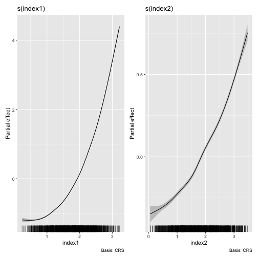
Residuals and fitted values
We can use the augment method to obtain the residuals
and the fitted values from an estimated SMI model.
## Obtain residuals and fitted values
augment(x = smimodel_ppr)
#> # A tibble: 1,200 × 3
#>    Index   .resid .fitted
#>    <int>    <dbl>   <dbl>
#>  1     6  0.0566    0.757
#>  2     7 -0.0397    1.50
#>  3     8 -0.0552    3.78
#>  4     9  0.0499    1.78
#>  5    10  0.155     1.88
#>  6    11 -0.145     3.70
#>  7    12  0.200     2.16
#>  8    13 -0.00571   2.20
#>  9    14 -0.0585    2.78
#> 10    15  0.0690    0.588
#> # ℹ 1,190 more rows
Forecasts on a test set
Based on an estimated SMI model, we obtain forecasts/predictions on a
test set as below, using the predict method.
## Obtain forecasts on the test set
preds = predict(object = smimodel_ppr, newdata = sim_test)
preds$.predict
#>          1          2          3          4          5          6          7          8          9
#> 3.45875259 1.52227838 0.52881104 2.24035158 1.12107147 1.37713685 3.45942510 1.29280288 1.30480760
#>         10         11         12         13         14         15         16         17         18
#> 0.76693416 0.94033375 1.69198167 1.19066341 1.31326856 1.62227903 2.32393332 0.83445703 1.04508990
#>         19         20         21         22         23         24         25         26         27
#> 1.18655331 4.77834376 0.61094061 1.14584964 0.79738240 1.40808298 2.33526200 0.17577515 0.55496943
#>         28         29         30         31         32         33         34         35         36
#> 0.36529819 0.86680931 0.58204728 0.07682039 0.12715469 0.59371085 2.34226095 0.88236602 0.31311292
#>         37         38         39         40         41         42         43         44         45
#> 0.47272680 0.98719807 1.08509641 1.63224918 1.08438592 0.94669238 0.69782251 0.29352743 1.42720367
#>         46         47         48         49         50         51         52         53         54
#> 1.80572138 1.56637665 1.60908623 0.46992486 0.52987039 1.75371557 0.35670514 0.52323854 2.84421134
#>         55         56         57         58         59         60         61         62         63
#> 1.52535348 1.21157098 1.57454092 0.35167609 0.81628181 1.16983691 0.14744439 0.76252668 3.59290968
#>         64         65         66         67         68         69         70         71         72
#> 0.41181444 2.45049844 1.07340894 0.95589469 2.55008954 0.60641501 3.72815494 1.90521972 2.62653129
#>         73         74         75         76         77         78         79         80         81
#> 2.97443784 1.17261901 1.32266114 0.58847194 1.53256266 2.14620254 1.74196253 2.66079827 0.79429653
#>         82         83         84         85         86         87         88         89         90
#> 2.20897818 1.95718405 1.04773411 1.37572254 2.27213107 1.86737728 0.84856583 2.17397767 1.42471476
#>         91         92         93         94         95         96         97         98         99
#> 0.92667153 2.26161088 2.21898501 3.09128273 2.79447124 0.60599090 1.10399804 1.38587451 1.84832772
#>        100        101        102        103        104        105        106        107        108
#> 2.95928627 1.75660705 0.83714657 0.44664008 1.24110982 0.44727137 0.43799614 0.43482032 1.11403760
#>        109        110        111        112        113        114        115        116        117
#> 0.90800010 0.98409355 0.77391461 0.92785753 1.44316813 0.53590956 0.70992483 0.71795358 1.41767391
#>        118        119        120        121        122        123        124        125        126
#> 1.35755259 2.13572836 2.08429360 2.88077416 0.93061594 2.19668318 0.26132355 1.22310358 1.28597904
#>        127        128        129        130        131        132        133        134        135
#> 0.54794253 1.30397046 1.46474006 1.18312452 0.66352232 1.22851353 2.41435557 2.60599716 2.59239098
#>        136        137        138        139        140        141        142        143        144
#> 0.97740761 1.39710803 1.03604458 0.73902008 1.11037088 2.98249685 1.16392033 1.56621624 2.29963520
#>        145        146        147        148        149        150        151        152        153
#> 1.45009245 1.01222387 0.19617259 0.24803096 0.17703054 0.24552278 0.11939235 0.06335250 0.78697563
#>        154        155        156        157        158        159        160        161        162
#> 0.77510661 0.44432578 2.11483463 0.36391308 1.84129095 1.72201999 0.56247570 0.86526871 0.15401982
#>        163        164        165        166        167        168        169        170        171
#> 0.86083789 0.36209679 0.16949950 0.38394360 0.08912956 0.44100934 0.88294634 1.29236413 2.58720558
#>        172        173        174        175        176        177        178        179        180
#> 1.48371732 3.04050479 1.20272911 1.04586676 2.14226125 0.44197929 2.79409719 0.52716239 1.55409562
#>        181        182        183        184        185        186        187        188        189
#> 1.42580960 0.36626185 2.72545139 0.29608435 0.87043136 2.92144635 1.94118373 1.64383166 1.23771152
#>        190        191        192        193        194        195        196        197        198
#> 0.96011483 2.37079432 2.37095016 1.44371807 0.58065932 0.37881098 0.50417286 0.34462475 0.18876236
#>        199        200
#> 0.20226401 0.26617350
Once we obtain forecasts/predictions, we can evaluate the forecasting/predictive performance of the estimated SMI model by calculating forecast/prediction error measurements as desired.
Tuning for penalty parameters
The estimation of a SMI model involves solving an optimisation problem, where the sum of squared errors of the model plus two penalty terms (an L0 penalty and an L2 (ridge) penalty) is minimised subject to a set of constraints. Thus, two penalty parameters and corresponding to the L0 and L2 penalties respectively should be chosen when estimating a SMI model.
In the previous example, all the SMI models were fitted using the
default penalty parameter values provided in the function:
and
.
To fit a SMI model with simultaneous parameter tuning, we can use the
function greedy_smimodel(), which performs a greedy search
over a partially data-derived grid of possible penalty parameter
combinations
(,
),
and fits the SMI model using the best (lowest validation set MSE)
penalty parameter combination. In this case, we need to provide a
validation set, which is separate from the training data set.
Therefore, let’s split our original training set in the above example into two parts again to obtain a validation set.
# New training set
sim_train_new <- sim_data[1:1000, ]

# Validation set
sim_val_new <- sim_data[1001:1200, ]
Next, we can estimate the SMI model with simultaneous penalty parameter tuning as follows. Here, we use the initialisation option “ppr” just to demonstrate the functionality.
## Estimating SMI model with penalty parameter tuning
smimodel_ppr_tune <- greedy_smimodel(data = sim_train_new,
                                     val.data = sim_val_new,
                                     yvar = "y",
                                     index.vars = index.vars,
                                     initialise = "ppr")
# Fitted optimal SMI model
smimodel_ppr_tune$fit[[1]]$best
#> SMI Model Fit:
#> Index coefficients:
#> 6 x 3 sparse Matrix of class "dgCMatrix"
#>          index1 index2 index3
#> x_000 0.4632129      .      .
#> x_001 0.3058459      .      .
#> x_002 .              .      1
#> x_003 0.2309412      .      .
#> x_004 .              .      .
#> x_005 .              1      .
#>
#> Response variable:
#> [1] "y"
#>
#> Index variables:
#> [1] "x_000" "x_001" "x_002" "x_003" "x_004" "x_005"
#>
#> Spline variables (non-index):
#> NULL
#>
#> Linear variables:
#> NULL
#>
#> GAM Fit:
#> Family: gaussian
#> Link function: identity
#>
#> Formula:
#> y ~ s(index1, bs = "cr") + s(index2, bs = "cr") + s(index3, bs = "cr")
#>
#> Estimated degrees of freedom:
#> 8.43 4.30 2.99  total = 16.72
#>
#> REML score: -945.3404
## Selected penalty parameter combination
smimodel_ppr_tune$fit[[1]]$best_lambdas
#> [1] 0.01356766 0.01000000
Here the selected penalty parameter combination is .